Better Binary Quantization (BBQ) in Lucene and Elasticsearch

Embedding models output float32 vectors, often too large for efficient processing and practical apps. Elasticsearch supports int8 scalar quantization to reduce vector size while preserving performance. Other methods reduce retrieval quality and are impractical for real world use. In Elasticsearch 8.16 and Lucene, we introduced Better Binary Quantization (BBQ), a new approach developed from insights drawn from a recent technique - dubbed “RaBitQ” - proposed by researchers from Nanyang Technological University, Singapore.

BBQ is a leap forward in quantization for Lucene and Elasticsearch, reducing float32 dimensions to bits, delivering ~95% memory reduction while maintaining high ranking quality. BBQ outperforms traditional approaches like Product Quantization (PQ) in indexing speed (20-30x less quantization time), query speed (2-5x faster queries), with no additional loss in accuracy.

In this blog, we will explore BBQ in Lucene and Elasticsearch, focusing on recall, efficient bitwise operations, and optimized storage for fast, accurate vector search.

What does the "better" in Better Binary Quantization mean?

In Elasticsearch 8.16 and in Lucene, we have introduced what we call "Better Binary Quantization". Naive binary quantization is exceptionally lossy and achieving adequate recall requires gathering 10x or 100x additional neighbors to rerank. This just doesn't cut it.

In comes Better Binary Quantization! Here are some of the significant differences between Better Binary Quantization and naive binary quantization:

• All vectors are normalized around a centroid. This unlocks some nice properties in quantization.
• Multiple error correction values are stored. Some of these corrections are for the centroid normalization, some are for the quantization.
• Asymmetric quantization. Here, while the vectors themselves are stored as single bit values, queries are only quantized down to int4. This significantly increases search quality at no additional cost in storage.
• Bit-wise operations for fast search. The query vectors are quantized and transformed in such a way that allows for efficient bit-wise operations.

Indexing with better binary quantization

Indexing is simple. Remember, Lucene builds individual read only segments. As vectors come in for a new segment the centroid is incrementally calculated. Then once the segment is flushed, each vector is normalized around the centroid and quantized.

Here is a small example:

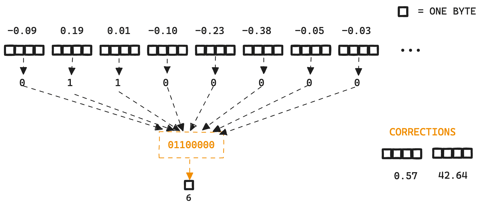
When quantizing down to the bit level, 8 floating point values are transformed into a single 8bit byte.

Then, each of the bits are packed into a byte and stored in the segment along with any error correction values required for the vector similarity chosen.

For each vector, bytes stored are dims/8 number of bytes and then any error correction values; 2 floating point values for Euclidean, or 3 for dot product.

A quick side quest to talk about how we handle merging

When segments are merged, we can take advantage of the previously calculated centroids. Simply doing a weighted average of the centroids and then re-quantizing the vectors around the new centroid.

What gets tricky is ensuring HNSW graph quality and allowing the graph to be built with the quantized vectors. What's the point of quantizing if you still need all the memory to build the index?!

In addition to appending vectors to the existing largest HNSW graph, we need to ensure vector scoring can take advantage of asymmetric quantization. HNSW has multiple scoring steps: one for the initial collection of neighbors, and another for ensuring only diverse neighbors are connected. In order to efficiently use asymmetric quantization, we create a temporary file of all vectors quantized as 4bit query vectors.

So, as a vector is added to the graph we first:

• Get the already quantized query vector that is stored in the temporary file.
• Search the graph as normal using the already existing bit vectors.
• Once we have the neighbors, diversity and reverse-link scoring can be done with the previously int4 quantized values.

After the merge is complete, the temporary file is removed leaving only the bit quantized vectors.

The temporary file stores each query vector as an int4 byte array which takes dims/2 number of bytes, some floating point error correction values (3 for Euclidean, 4 for dot product), and a short value for the sum of the vector dimensions.

Asymmetric quantization, the interesting bits

I have mentioned asymmetric quantization and how we lay out the queries for graph building. But, how are the vectors actually transformed? How does it work?

The "asymmetric" part is straight forward. We quantize the query vectors to a higher fidelity. So, doc values are bit quantized and query vectors are int4 quantized. What gets a bit more interesting is how these quantized vectors are transformed for fast queries.

Taking our example vector from above, we can quantize it to int4 centered around the centroid.

With the quantized vector in hand, this is where the fun begins. So we can translate the vector comparisons to a bitwise dot product, the bits are shifted.

Its probably better to just visualize what is happening:

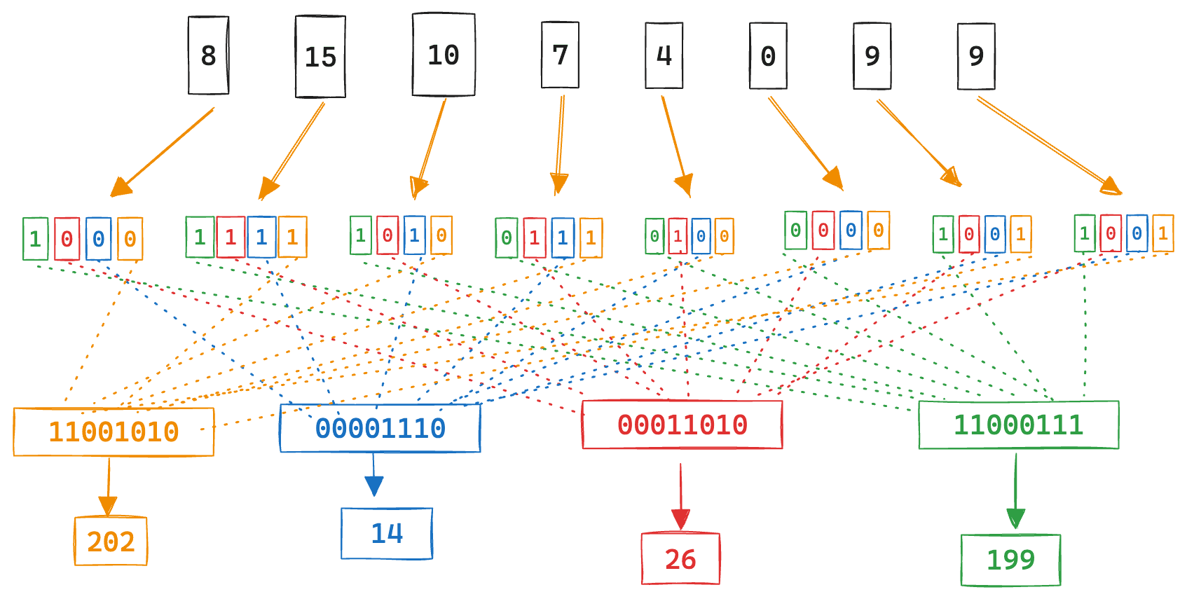
Here, each int4 quantized value has its relative positional bits shifted to a single byte. Note how all the first bits are packed together first, then the second bits, and so on.

But how does this actually translate to dot product? Remember, dot product is the sum of the component products. For the above example, let's write this fully out:

We can see that its simply the summation of the query components where the stored vector bits are 1. And since all numbers are just bits, when expressed using a binary expansion, we can move things around a bit to take advantage of bitwise operations.

The bits that will be flipped after the $\&$ will be the individual bits of the numbers that contribute to the dot product. In this case 15 and 10.

Now we can count the bits, shift and sum back together. We can see that all the bits that are left over are the positional bits for 15 and 10.

Same answer as summing the dimensions directly.

Here is the example but simplifed java code:

byte[] bits = new byte[]{6};
byte[] queryBits = new byte[]{202, 14, 26, 199};
for (int i = 0; i < 4; i++) {
  sum += Integer.bitCount(bits[0] & queryBits[i] & 0xFF) << i;
}

Alright, show me the numbers

We have done extensive testing with BBQ both in Lucene and Elasticsearch directly. Here are some of the results:

Lucene benchmarking

The benchmarking here is done over three datasets: E5-small, CohereV3, and CohereV2. Here, each element indicates recall@100 with oversampling by [1, 1.5, 2, 3, 4, 5].

E5-small

This is 500k vectors for E5-small built from the quora dataset.

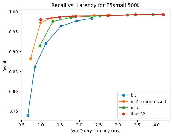
It's sort of mind blowing that we get recall of 74% with only a single bit precision. Since the number of dimensions are fewer, the BBQ distance calculation isn't that much faster than our optimized int4.

CohereV3

This is 1M 1024 dimensional vectors, using the CohereV3 model.

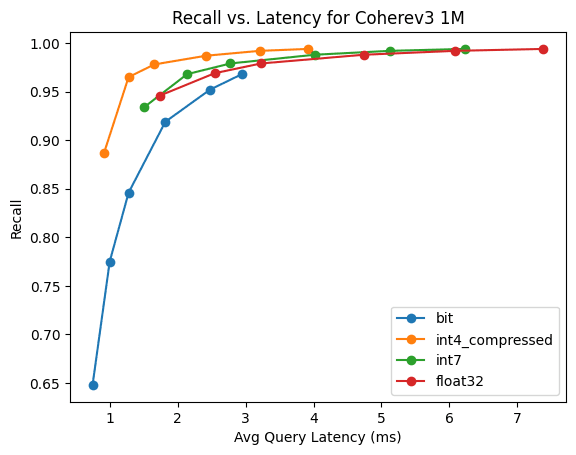
Here, 1bit quantization and HNSW gets above 90% recall with only 3x oversampling.

CohereV2

This is 1M 768 dimensional vectors, using the CohereV2 model and max inner product similarity.

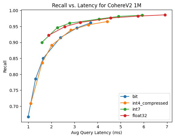
It's really interesting to see how much BBQ and int4 are in lock-step with this benchmark. Its neat that BBQ can get such high recall with inner-product similarity with only 3x oversampling.

Larger scale Elasticsearch benchmarking

As referenced in our larger scale vector search blog we have a rally track for larger scale vector search benchmarking.

This data set has 138M floating point vectors of 1024 dimensions. Without any quantization, this would require around 535 GB of memory with HNSW. With better-binary-quantization, the estimate drops to around 19GB.

For this test, we used a single 64GB node in Elastic cloud with the following track parameters:

{
        "mapping_type": "vectors-only",
        "vector_index_type": "bbq_hnsw",
        "number_of_shards": 2,
        "initial_indexing_bulk_indexing_clients": 12,
        "standalone_search_clients": 8,
        "aggressive_merge_policy": true,
        "search_ops": [[10, 20, 0], [10, 20, 20], [10, 50, 0], [10, 50, 20], [10, 50, 50], [10, 100, 0], [10, 100, 20], [10, 100, 50], [10, 100, 100], [10, 200, 0], [10, 200, 20], [10, 200, 50], [10, 200, 100], [10, 200, 200], [10, 500, 0], [10, 500, 20], [10, 500, 50],[10, 500, 100],[10, 500, 200],[10, 500, 500],[10, 1000, 0], [10, 1000, 20], [10, 1000, 50], [10, 1000, 100], [10, 1000, 200], [10, 1000, 500], [10, 1000, 1000]]
}

Important note, if you want to replicate, it will take significant time to download all the data and requires over 4TB of disk space. The reason for all the additional disk space is that this dataset also contains text fields, and you need diskspace for both the compressed files and their inflated size.

The parameters are as follows:

• k is the number of neighbors to search for
• num_candidates is the number of candidates used to explore per shard in HNSW
• rerank is the number of candidates to rerank, so we will gather that many values per shard, collect the total rerank size and then rescore the top k values with the raw float32 vectors.

For indexing time, it took around 12 hours. And instead of showing all the results, here are three interesting ones:

This shows the importance of balancing recall, oversampling, reranking and latency. Obviously, each needs to be tuned for your specific use case, but considering this was impossible before and now we have 138M vectors in a single node, it's pretty cool.

Conclusion

Thank you for taking a bit of time and reading about Better Binary Quantization. Originally being from Alabama and now living in South Carolina, BBQ already held a special place in my life. Now, I have more reason to love BBQ!

We will release this as tech-preview in 8.16, or in serverless right now. To use this, just set your dense_vector.index_type as bbq_hnsw or bbq_flat in Elasticsearch.

Related content

Vector DatabaseLucene+1

October 22, 2024

RaBitQ binary quantization 101

Understand the most critical components of RaBitQ binary quantization, how it works and its benefits. This guide also covers the math behind the quantization and examples.

JW

By: John Wagster

Lucene

October 14, 2024

Apache Lucene 10 is out! Improvements to Lucene's hardware efficiency & more

Apache Lucene 10 was just released, with a focus on hardware efficiency! Check out the main release highlights.

AG

By: Adrien Grand

Lucene

December 7, 2023

Apache Lucene 9.9, the fastest Lucene release ever

Lucene 9.9 brings major speedups to query evaluation. Here are the performance improvements observed in nightly benchmarks & optimization resources.

AG

By: Adrien Grand

Vector DatabaseLucene

June 26, 2024

Elasticsearch vs. OpenSearch: Vector Search Performance Comparison

Elasticsearch is out-of-the-box 2x–12x faster than OpenSearch for vector search

US

By: Ugo Sangiorgi

Lucene

September 1, 2023

Bringing maximum-inner-product into Lucene

Explore how we brought maximum-inner-product into Lucene and the investigations undertaken to ensure its support.

BT

By: Benjamin Trent