Map custom regions with reverse geocoding
editMap custom regions with reverse geocoding
editMaps comes with predefined regions that allow you to quickly visualize regions by metrics. Maps also offers the ability to map your own regions. You can use any region data you’d like, as long as your source data contains an identifier for the corresponding region.
But how can you map regions when your source data does not contain a region identifier? This is where reverse geocoding comes in. Reverse geocoding is the process of assigning a region identifier to a feature based on its location.
In this tutorial, you’ll use reverse geocoding to visualize United States Census Bureau Combined Statistical Area (CSA) regions by web traffic.
You’ll learn to:
- Upload custom regions.
- Reverse geocode with the Elasticsearch enrich processor.
- Create a map and visualize CSA regions by web traffic.
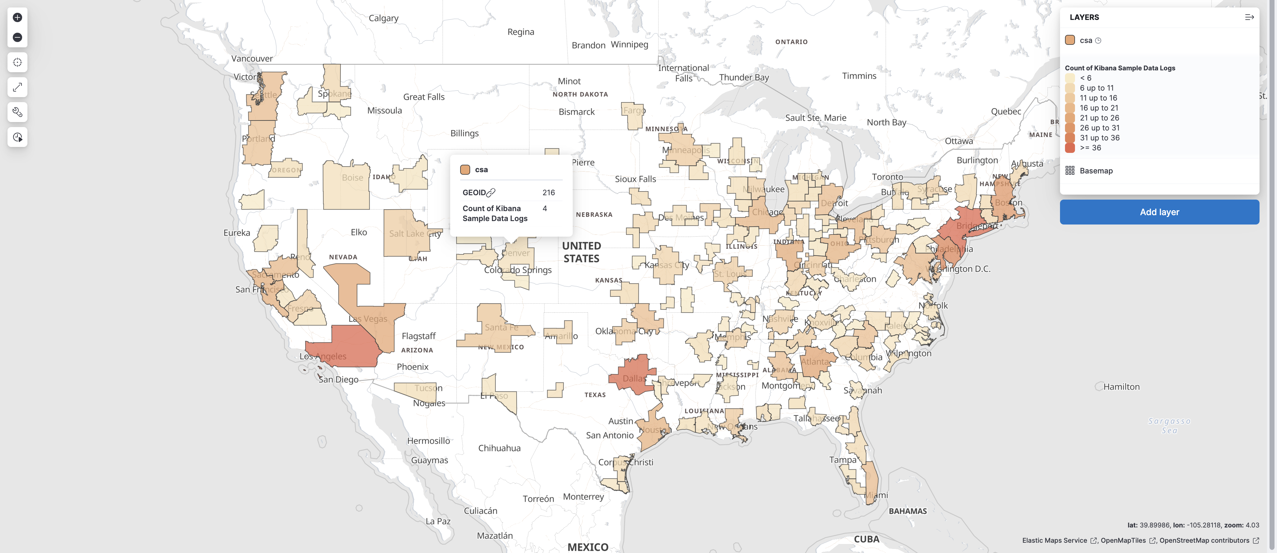
When you complete this tutorial, you’ll have a map that looks like this:
Step 1: Index web traffic data
editGeoIP is a common way of transforming an IP address to a longitude and latitude. GeoIP is roughly accurate on the city level globally and neighborhood level in selected countries. It’s not as good as an actual GPS location from your phone, but it’s much more precise than just a country, state, or province.
You’ll use the web logs sample data set that comes with Kibana for this tutorial. Web logs sample data set has longitude and latitude. If your web log data does not contain longitude and latitude, use GeoIP processor to transform an IP address into a geo_point field.
To install web logs sample data set:
- On the home page, click Try sample data.
- Expand Other sample data sets.
- On the Sample web logs card, click Add data.
Step 2: Index Combined Statistical Area (CSA) regions
editGeoIP level of detail is very useful for driving decision-making. For example, say you want to spin up a marketing campaign based on the locations of your users or show executive stakeholders which metro areas are experiencing an uptick of traffic.
That kind of scale in the United States is often captured with what the Census Bureau calls the Combined Statistical Area (CSA). CSA is roughly equivalent with how people intuitively think of which urban area they live in. It does not necessarily coincide with state or city boundaries.
CSAs generally share the same telecom providers and ad networks. New fast food franchises expand to a CSA rather than a particular city or municipality. Basically, people in the same CSA shop in the same IKEA.
To get the CSA boundary data:
-
Go to the Census Bureau’s website and download the
cb_2018_us_csa_500k.zipfile. - Uncompress the zip file.
- In Kibana, open the main menu, and click Maps.
- Click Create map.
- Click Add layer.
- Click Upload file.
-
Use the file chooser to select the
.shpfile from the CSA shapefile folder. -
Use the
.dbffile chooser to select the.dbffile from the CSA shapefile folder. -
Use the
.prjfile chooser to select the.prjfile from the CSA shapefile folder. -
Use the
.shxfile chooser to select the.shxfile from the CSA shapefile folder. - Set index name to csa and click Import file.
- When importing is complete, click Add as document layer.
-
Add Tooltip fields:
- Click + Add to open the field select.
- Select NAME, GEOID, and AFFGEOID.
- Click Add.
- Click Keep changes.
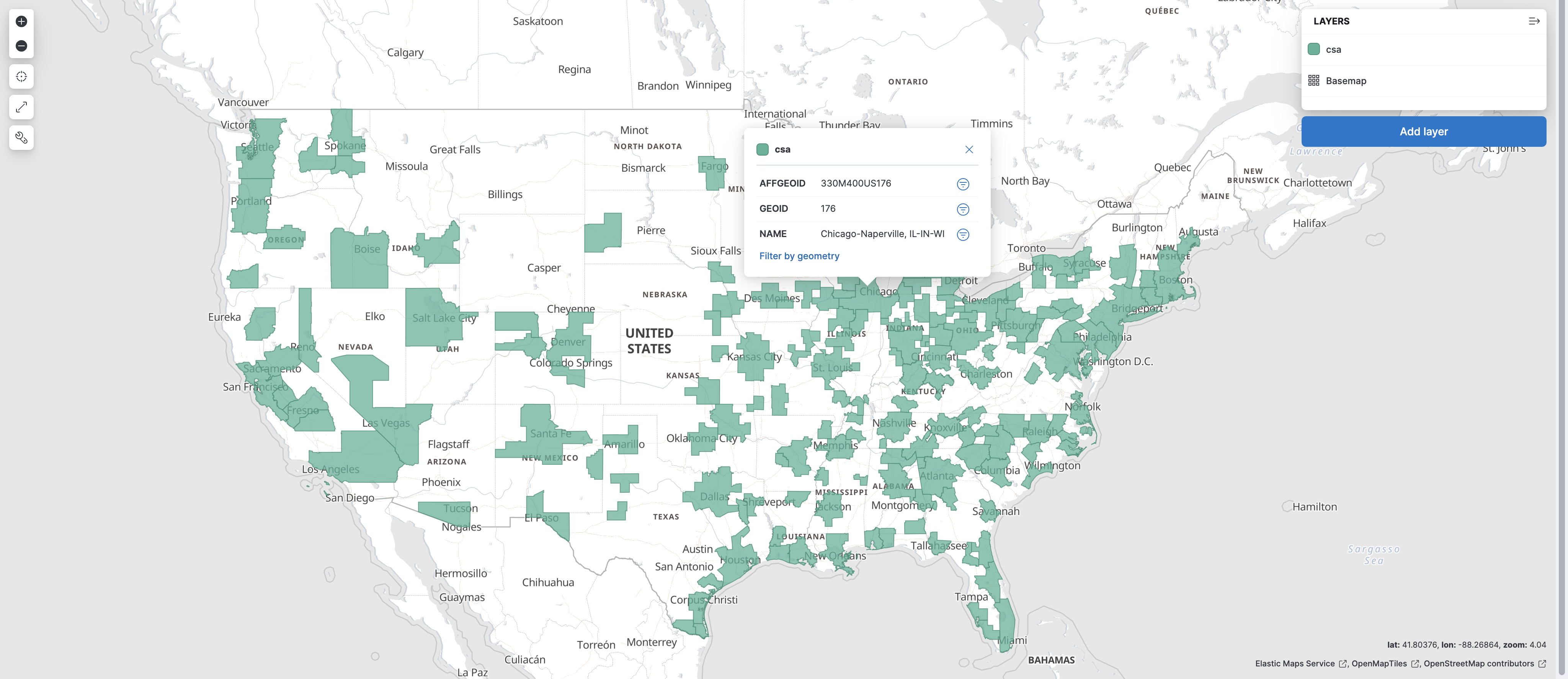
Looking at the map, you get a sense of what constitutes a metro area in the eyes of the Census Bureau.
Step 3: Reverse geocoding
editTo visualize CSA regions by web log traffic, the web log traffic must contain a CSA region identifier. You’ll use Elasticsearch enrich processor to add CSA region identifiers to the web logs sample data set. You can skip this step if your source data already contains region identifiers.
- Open the main menu, and then click Dev Tools.
-
In Console, create a geo_match enrichment policy:
PUT /_enrich/policy/csa_lookup { "geo_match": { "indices": "csa", "match_field": "geometry", "enrich_fields": [ "GEOID", "NAME"] } } -
To initialize the policy, run:
POST /_enrich/policy/csa_lookup/_execute
-
To create a ingest pipeline, run:
PUT _ingest/pipeline/lonlat-to-csa { "description": "Reverse geocode longitude-latitude to combined statistical area", "processors": [ { "enrich": { "field": "geo.coordinates", "policy_name": "csa_lookup", "target_field": "csa", "ignore_missing": true, "ignore_failure": true, "description": "Lookup the csa identifier" } }, { "remove": { "field": "csa.geometry", "ignore_missing": true, "ignore_failure": true, "description": "Remove the shape field" } } ] } -
To update your existing data, run:
POST kibana_sample_data_logs/_update_by_query?pipeline=lonlat-to-csa
-
To run the pipeline on new documents at ingest, run:
PUT kibana_sample_data_logs/_settings { "index": { "default_pipeline": "lonlat-to-csa" } } - Open the main menu, and click Discover.
- Set the data view to Kibana Sample Data Logs.
- Open the time filter, and set the time range to the last 30 days.
-
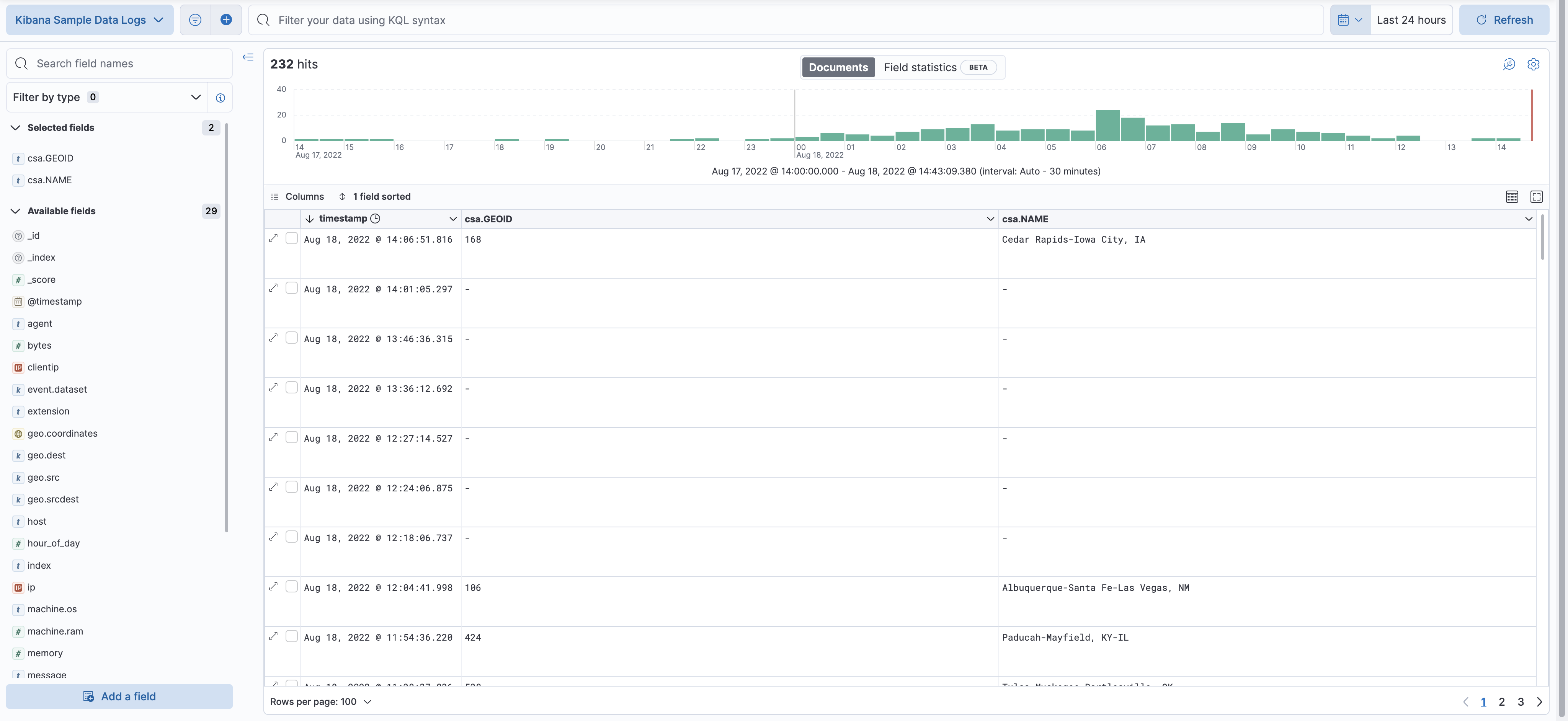
Scan through the list of Available fields until you find the
csa.GEOIDfield. You can also search for the field by name. -
Click
 to toggle the field into the document table.
- Find the csa.NAME field and add it to your document table.
Your web log data now contains csa.GEOID and csa.NAME fields from the matching csa region. Web log traffic not contained in a CSA region does not have values for csa.GEOID and csa.NAME fields.
Step 4: Visualize Combined Statistical Area (CSA) regions by web traffic
editNow that our web traffic contains CSA region identifiers, you’ll visualize CSA regions by web traffic.
- Open the main menu, and click Maps.
- Click Create map.
- Click Add layer.
- Click Choropleth.
-
For Boundaries source:
- Select Points, lines, and polygons from Elasticsearch.
- Set Data view to csa.
- Set Join field to GEOID.
-
For Statistics source:
- Set Data view to Kibana Sample Data Logs.
- Set Join field to csa.GEOID.keyword.
- Click Add and continue.
- Scroll to Layer Style and Set Label to Fixed.
- Click Keep changes.
-
Save the map.
- Give the map a title.
- Under Add to dashboard, select None.
- Click Save and add to library.
Congratulations! You have completed the tutorial and have the recipe for visualizing custom regions. You can now try replicating this same analysis with your own data.