WARNING: Version 5.6 of Elasticsearch has passed its EOL date.
This documentation is no longer being maintained and may be removed. If you are running this version, we strongly advise you to upgrade. For the latest information, see the current release documentation.
Serial Differencing Aggregation
editSerial Differencing Aggregation
editThis functionality is in technical preview and may be changed or removed in a future release. Elastic will work to fix any issues, but features in technical preview are not subject to the support SLA of official GA features.
Serial differencing is a technique where values in a time series are subtracted from itself at different time lags or periods. For example, the datapoint f(x) = f(xt) - f(xt-n), where n is the period being used.
A period of 1 is equivalent to a derivative with no time normalization: it is simply the change from one point to the next. Single periods are useful for removing constant, linear trends.
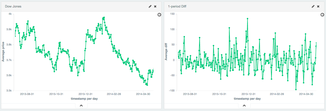
Single periods are also useful for transforming data into a stationary series. In this example, the Dow Jones is plotted over ~250 days. The raw data is not stationary, which would make it difficult to use with some techniques.
By calculating the first-difference, we de-trend the data (e.g. remove a constant, linear trend). We can see that the data becomes a stationary series (e.g. the first difference is randomly distributed around zero, and doesn’t seem to exhibit any pattern/behavior). The transformation reveals that the dataset is following a random-walk; the value is the previous value +/- a random amount. This insight allows selection of further tools for analysis.

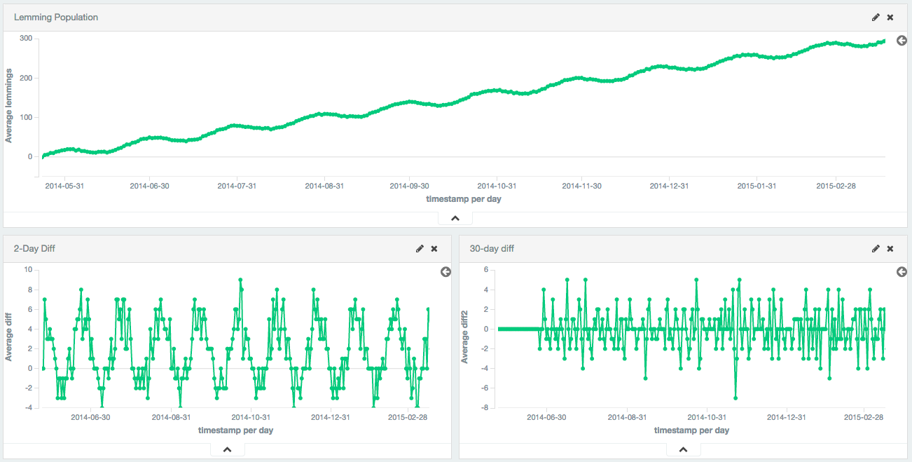
Larger periods can be used to remove seasonal / cyclic behavior. In this example, a population of lemmings was synthetically generated with a sine wave + constant linear trend + random noise. The sine wave has a period of 30 days.
The first-difference removes the constant trend, leaving just a sine wave. The 30th-difference is then applied to the first-difference to remove the cyclic behavior, leaving a stationary series which is amenable to other analysis.

Syntax
editA serial_diff aggregation looks like this in isolation:
{
    "serial_diff": {
        "buckets_path": "the_sum",
        "lag": "7"
    }
}
Table 13. serial_diff Parameters
| Parameter Name | Description | Required | Default Value |
|---|---|---|---|
|
Path to the metric of interest (see |
Required |
|
|
The historical bucket to subtract from the current value. E.g. a lag of 7 will subtract the current value from the value 7 buckets ago. Must be a positive, non-zero integer |
Optional |
|
|
Determines what should happen when a gap in the data is encountered. |
Optional |
|
|
Format to apply to the output value of this aggregation |
Optional |
|
serial_diff aggregations must be embedded inside of a histogram or date_histogram aggregation:
POST /_search
{
   "size": 0,
   "aggs": {
      "my_date_histo": {
         "date_histogram": {
            "field": "timestamp",
            "interval": "day"
         },
         "aggs": {
            "the_sum": {
               "sum": {
                  "field": "lemmings"
               }
            },
            "thirtieth_difference": {
               "serial_diff": {
                  "buckets_path": "the_sum",
                  "lag" : 30
               }
            }
         }
      }
   }
}
|
A |
|
|
A |
|
|
Finally, we specify a |
Serial differences are built by first specifying a histogram or date_histogram over a field. You can then optionally
add normal metrics, such as a sum, inside of that histogram. Finally, the serial_diff is embedded inside the histogram.
The buckets_path parameter is then used to "point" at one of the sibling metrics inside of the histogram (see
buckets_path Syntax for a description of the syntax for buckets_path.